Futures cumulative delta and market depth analysis
TL;DR
In a previous post a preliminary analysis of price data from Micro E-mini futures was made using volume traded per time window. In this post I go a step further, identifying buy/sell preponderance and better understanding the correlation of order flow and price trends.
Intro
The preliminary analysis made previously was not able to explain how an increased trading volume could account for both uptrend and downtrend in the price over time. Figure 1 below illustrates that situation, with areas highlighted as 1 corresponding to an uptrend, 2 to a downtrend and 3 an uptrend that is reversed to a downtrend.
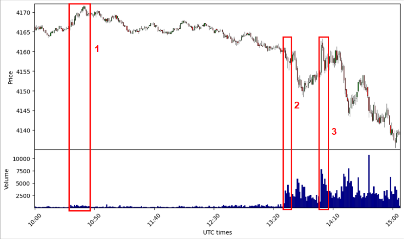 Figure 1: Volume increases, price trends
How could we distinguish the trade volume that pushes the price up from the one that pulls it down? One way to do this is by using tick data, on which every trade made is recorded, and the concept of market depth.
Getting data
Getting tick data via MetaTrader5 is done either pressing CTRL+U or the menu item View->Symbols, after which the window depicted in Figure 2 should appear.
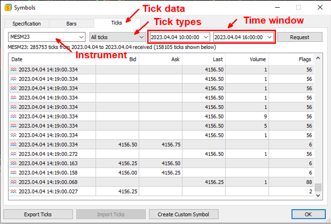 Figure 2: Capturing tick data
After switching to the Ticks tab, selecting the instrument (MESM23 at the time of writing), the All ticks dropdown menu option for ticks type and the desired time window, the ticks can be requested and exported to a local file. The first difference to the OHLC data used in the previous post is the amount of it: five hour of trading data, as used in the examples, have 300 OHLC records, one for each minute. In the tick data there is one record per trade made; in the most active moments of the data sample, there can be as many as 10,000 records in a minute.
By default, the tick data is saved as a tab separated text file and should have a structure similar to Figure 3 below.
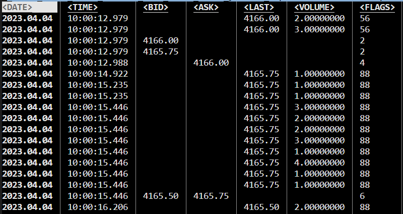 Figure 3: Raw tick data
The column representing the time in tick data has a precision of milliseconds and is relevant to sort the large amount of trades happening almost simultaneously. The <BID> column represents the best price one could get when selling a unit of the instrument at that given point in time. The <ASK> columns represents the best price one could pay for a unit of the instrument at that given point in time. Records with values on the either <BID> or <ASK> columns represent moments on which these prices have changed.
The columns <FLAGS> marks those changes as well: code 2 represents a change in <BID> price; code 4, represents a change in <ASK> price; and code 6, a change in both.
Records with values 56 or 88 in the <FLAGS> column represent, respectively, market orders executed for buying and selling units of the instrument. At time 10:00:10.979 two buy orders were executed, the first with volume of 2 units and the second, with 3 units.
Market depth
In order to contextualize the changes in price seen in the tick data, it is relevant to mention the concept of market depth (or depth of market, DOM). Figure 4 below is a snapshot of the sidebar item in MT5 when the menu item View->Depth Of Market is clicked.
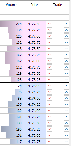
The central part of the picture, where the black line separates the red bars from the blue ones, is where the current <BID> and <ASK> prices are located. The blue bar closest to the central line is the current <BID>, $4,175.00; the red bar represents the current <ASK>, $4,175.25.
The values in the Volume column represent limit orders placed by traders at each price level and, in principle, reflect the market capacity to absorb market order made by other traders. Large volumes in each price level indicate the need for a very strong buy or sell activity in order to move the price.
The state of the DOM is dynamic, in the sense the as the market orders are executed or new limit orders are placed, the volumes of instrument units at each price level change, often modifying the <BID> and <ASK> prices.
An example of the influence the market order execution sequence has on the DOM can be inferred from the tick data on Figure 3. The <BID> price changed at 10:00:12.979 to $4,165.75 and the <ASK> price at 10:00:12.988 to $4,166.00.
After that, a series of sell deals were made in sequence between 10:00:14 and 10:00:15 with volumes between 1 and 4 units, all at the same price of $4,165.75. Right after this series of sells the <BID> and <ASK> prices change, decreasing to $4,165.50 and $4,165.75.
Each sell order executed at $4,165.75 consumes a certain amount of bid units available in the DOM. If there are no new limit orders at that price to replace those consumed, eventually all the bids will be consumed and the <BID> price will go down. This behavior is aligned with the intuition that if a large enough number of traders sell the instrument its price is driven down.
Volume delta
In order to get a more precise sense of how the sequence of executed orders is flowing, there is the need to use something other than the combined volume indicator, with counts together buy and sell traded units. The cumulative delta, which indicates whether there was a preponderance of buying or selling trades at a given time window, is an alternative to quantify these imbalances and help to correlate order flow and price trends.
The volume delta is calculated here over a time window by subtracting the volume of sell order from the volume of buy order. If the sell volume is higher in that period, the delta will be negative; if the buy volume is higher, the delta will be positive.
The Python code below extends the code from the previous post by reading tick data, calculating the volume delta for each 1-minute time window and merging it with the OHLC data used previously.
"""Cumulative volume calculation and plotting"""
import sys
import mplfinance as mpf
import pandas as pd

TICK_BUY = 56
TICK_SELL = 88

tick_data_filename = sys.argv[1]

print(f"Loading tick data from {tick_data_filename}...")
tick_data = pd.read_csv(tick_data_filename, sep="\t")

tick_data.columns = [
    "date",
    "time",
    "bid",
    "ask",
    "last",
    "volume",
    "flags",
]

# Replace dots in date, concatenate date and time strings
tick_data["date"] = tick_data["date"].str.replace(".", "-", regex=False)
tick_data["datetime_str"] = (
    tick_data["date"] + [" "] * len(tick_data) + tick_data["time"]
)

# Convert to datetime
tick_data["datetime"] = pd.to_datetime(tick_data["datetime_str"], unit="ns")

# Retrieve date components
tick_data["year"] = tick_data["datetime"].dt.year
tick_data["month"] = tick_data["datetime"].dt.month
tick_data["day"] = tick_data["datetime"].dt.day
tick_data["hour"] = tick_data["datetime"].dt.hour
tick_data["minute"] = tick_data["datetime"].dt.minute

# Assign negative values for sell volumes
tick_data.loc[tick_data["flags"] == TICK_SELL, "volume"] = (
    -1 * tick_data.loc[tick_data["flags"] == TICK_SELL, "volume"]
)

# Group orders by minute and calculate delta
grouped = tick_data.groupby(["year", "month", "day", "hour", "minute"])["volume"].sum()
end_result = grouped.reset_index(name="delta")

ohlc_filename = sys.argv[2]

print(f"Loading candle data from {ohlc_filename}...")
ohlc_data = pd.read_csv(ohlc_filename, sep="\t")
ohlc_data.columns = [
    "date",
    "time",
    "open",
    "high",
    "low",
    "close",
    "tick_volume",
    "volume",
    "spread",
]

ohlc_data["date"].str.replace('.','-', regex=False)
ohlc_data["datetime_str"] = ohlc_data['date'] + [' '] * len(ohlc_data) +  ohlc_data['time']

ohlc_data["datetime"] = pd.to_datetime(ohlc_data["datetime_str"])

# Retrieve date components
ohlc_data["year"] = ohlc_data["datetime"].dt.year
ohlc_data["month"] = ohlc_data["datetime"].dt.month
ohlc_data["day"] = ohlc_data["datetime"].dt.day
ohlc_data["hour"] = ohlc_data["datetime"].dt.hour
ohlc_data["minute"] = ohlc_data["datetime"].dt.minute

ohlc_data = ohlc_data.merge(end_result, on=["year", "month", "day", "hour", "minute"])

ohlc_data = ohlc_data[["datetime","open", "high", "low", "close", "delta"]]
ohlc_data.columns = ["datetime","open", "high", "low", "close", "volume"]

# Adjust volume ylim
delta_plot = mpf.make_addplot(
    [0],
    type="bar",
    panel=1,
    secondary_y=False,
    ylim=(ohlc_data["volume"].min() * 1.2, ohlc_data["volume"].max() * 1.2),
)

ohlc_data.set_index("datetime", inplace=True)

market_colors = mpf.make_marketcolors(
    up="green", down="red", volume={"up": "green", "down": "red"}
)
custom_style = mpf.make_mpf_style(marketcolors=market_colors)

print("Saving plot...")
mpf.plot(
    ohlc_data[["open", "high", "low", "close", "volume"]],
    tight_layout=True,
    volume=True,
    type="candle",
    figratio=(16, 9),
    style=custom_style,
    addplot=delta_plot,
    savefig="candle_cumulative_delta_M1.png",
    xlabel="UTC times",
    ylabel_lower="Delta"
)
The resulting plot can be seen in Figure 5 below; of special interest is the volume graph of having green bars for minutes with buy preponderance and red bars for minutes with sell preponderance.
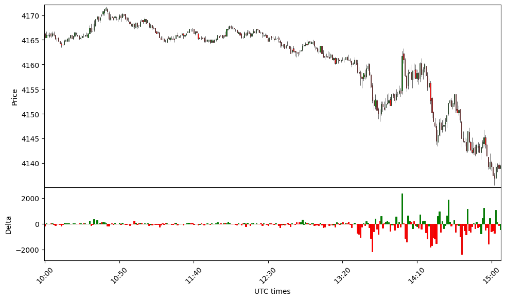 Figure 5: Cumulative delta, price trends
High level analysis
At a glance the delta values seem to match well with the price trends, in the sense that strong sell activity during a 1-minute time window often indicates that the price is falling. Inversely, marked preponderance of buy orders is often associated with raising prices.
If we zoom into a smaller time window to examine what the delta can tell about the price swing around the 14:00 mark, we can see that effect up close. Figure 6 below illustrates that.
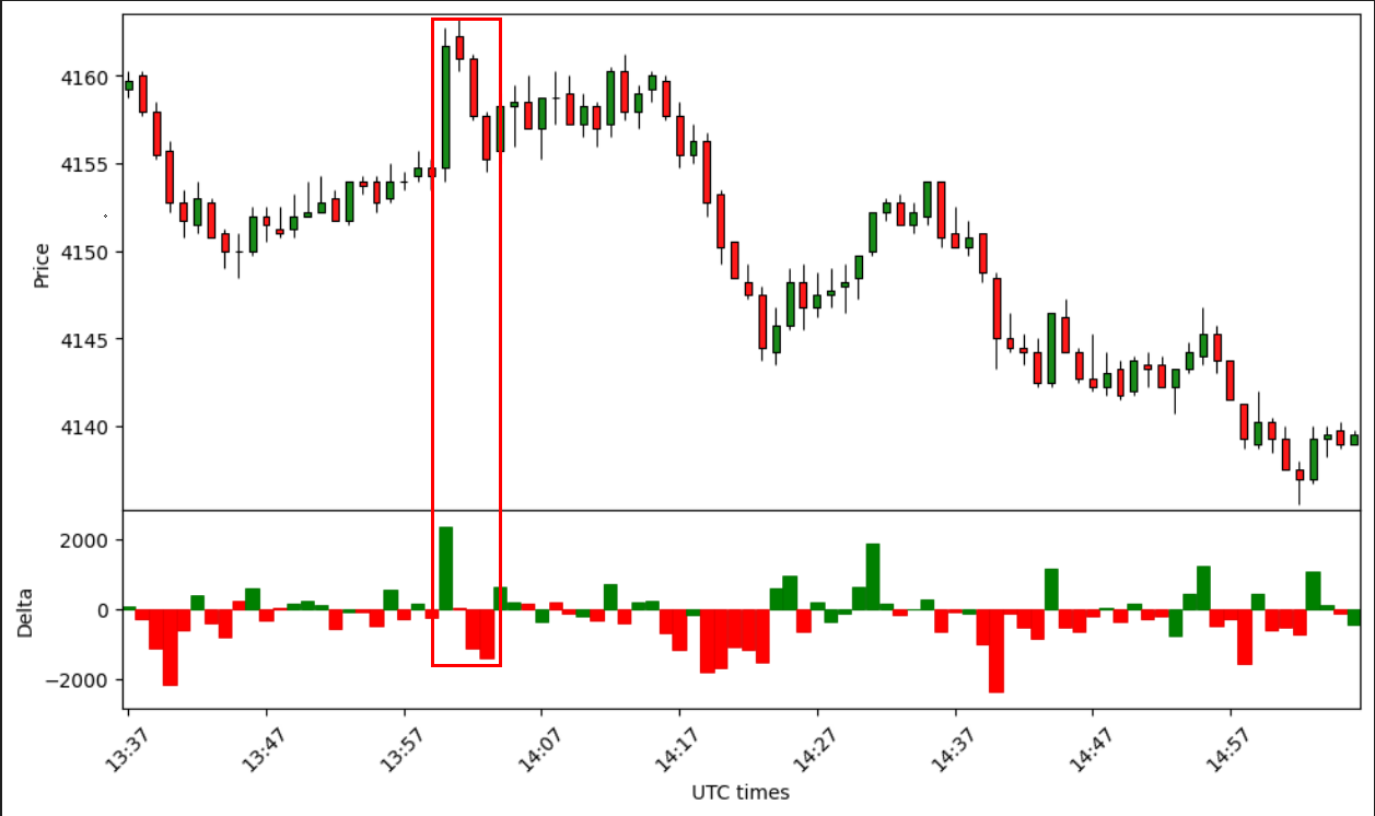 Figure 6: Correlation of delta and price swings
The image indicates that the price variation is closely correlated to the delta value. A strong buy activity, producing a positive delta of large magnitude, occurs at the same minute when a sharp raise in price takes place. That is immediately followed by a reversal, when a strong sell activity happens together with a quick price fall.
With this new results we reach the goal of having a tool for a more detailed analysis of order flow impact in price. The next step would be to find ways to use these results in real trading operations, which will be the topic of upcoming posts.
Disclaimer
Futures and options trading has large potential rewards, but also large potential risk. You must be aware of the risks and be willing to accept them in order to invest in the futures and options markets. Do not trade with money you can not afford to lose. This post is neither a solicitation nor an offer to buy or sell futures or options. No representation is being made that any account will or is likely to achieve profits or losses similar to those discussed. The past performance of any trading system or methodology is not necessarily indicative of future results.
This post is provided for informational and educational purposes only. This material neither is, nor should be construed as an offer, solicitation, or recommendation to buy or sell any securities. Any investment decisions made by the reader through the use of this content is solely based on the reader independent analysis, taking into consideration their financial circumstances and risk tolerance. The author shall not be liable for any errors or for any actions taken in reliance thereon.
The references made to MT5 and AMP Global in this post do not represent a recommendation. I am not affiliated to neither platform, service nor their parent companies.